Optimizing multi-scale cut-offs with fractopo

This functionality is very much so a work-in-progress. Optimization of a power-law fit for continuous, “single-scale”, data is easily handled by the functionality provided by powerlaw but it does not directly translate to the required methods for multi-scale data where normalization of the complementary cumulative number (=ccm) has been done.

Initializing

import matplotlib as mpl
import matplotlib.pyplot as plt

# Load three networks, each digitized from a different scale of observation
from example_data import HASTHOLMEN_NETWORK, KB11_NETWORK, LIDAR_200K_NETOWORK

from fractopo import general
from fractopo.analysis import length_distributions

mpl.rcParams["figure.figsize"] = (5, 5)
mpl.rcParams["font.size"] = 8

Collect LengthDistributions into MultiLengthDistribution

networks = [KB11_NETWORK, HASTHOLMEN_NETWORK, LIDAR_200K_NETOWORK]

distributions = [netw.trace_length_distribution(azimuth_set=None) for netw in networks]

mld = length_distributions.MultiLengthDistribution(
    distributions=distributions,
    using_branches=False,
    fitter=length_distributions.scikit_linear_regression,
)

Use scipy.optimize.shgo to optimize cut-off values

# See https://docs.scipy.org/doc/scipy/reference/generated/scipy.optimize.shgo.html
# for potential keyword arguments to pass to the shgo call
# shgo_kwargs are passed as is to ``scipy.optimize.shgo``.
shgo_kwargs = dict(
    sampling_method="sobol",
)

# Choose loss function for optimization. Here r2 is chosen to get a visually
# sensible result but it is generally ill-suited for optimizing cut-offs of
# power-law distributions.
scorer = general.r2_scorer

# Returns new instance of MultiLengthDistribution
# with optimized cut-offs.
opt_result, opt_mld = mld.optimize_cut_offs(scorer=scorer)

# Use optimized MultiLengthDistribution to plot distributions and fit.
# automatic_cut_offs is given as False to use the optimized cut-offs added as
# attributes of the MultiLengthDistribution instance.
polyfit, fig, ax = opt_mld.plot_multi_length_distributions(
    automatic_cut_offs=False, scorer=scorer, plot_truncated_data=True
)

# Print some results
print(
    f"""
Optimized cut-offs:
{opt_result.optimize_result.x}
Resulting power-law exponent:
{opt_result.polyfit.m_value}
Resulting {scorer.__name__} score:
{opt_result.polyfit.score}
"""
)

# Visual plot setup
plt.tight_layout()

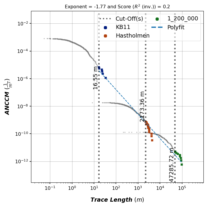
Optimized cut-offs:
[1.65542653e+01 2.17336026e+03 4.72857200e+04]
Resulting power-law exponent:
-1.7697755949276501
Resulting r2_scorer score:
0.1995943336682866