Plotting length distributions with fractopo

Initializing

from pprint import pprint

import matplotlib as mpl
import matplotlib.pyplot as plt

# Load kb11_network network from examples/example_data.py
from example_data import KB11_NETWORK

mpl.rcParams["figure.figsize"] = (5, 5)
mpl.rcParams["font.size"] = 8

Plotting length distribution plots of fracture traces and branches

Using Complementary Cumulative Number/Function

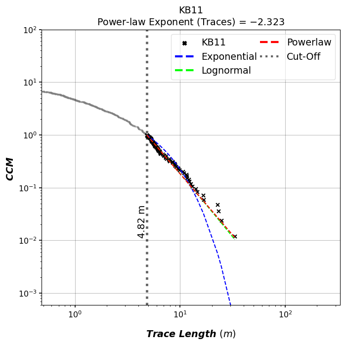
# Log-log plot of network trace length distribution
fit, fig, ax = KB11_NETWORK.plot_trace_lengths()

# Use matplotlib helpers to make sure plot fits in the gallery webpage!
# (Not required.)
plt.tight_layout()
plt.show()

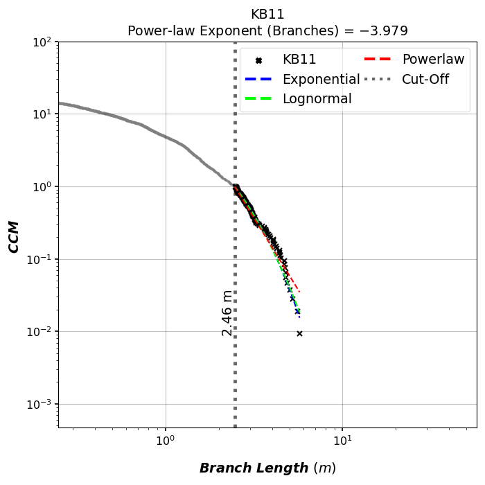
# Log-log plot of network branch length distribution
KB11_NETWORK.plot_branch_lengths()
plt.tight_layout()
plt.show()

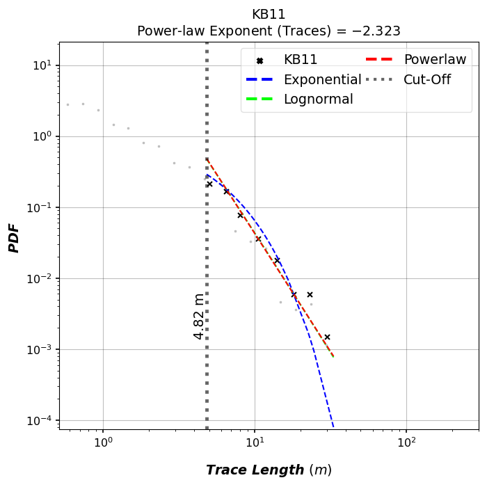
Using Probability Density Function

# Log-log plot of network trace length distribution
KB11_NETWORK.plot_trace_lengths(use_probability_density_function=True)

# Use matplotlib helpers to make sure plot fits in the gallery webpage!
# (Not required.)
plt.tight_layout()
plt.show()

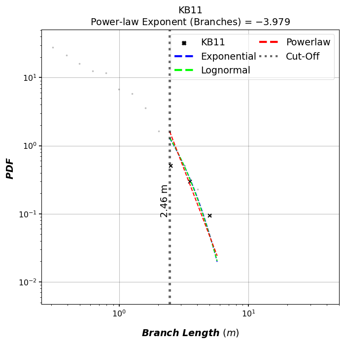
# Log-log plot of network branch length distribution
KB11_NETWORK.plot_branch_lengths(use_probability_density_function=True)
plt.tight_layout()
plt.show()

Numerical descriptions of fits are accessible as properties

# Use pprint for printing with prettier output
pprint(KB11_NETWORK.trace_lengths_powerlaw_fit_description)

{'trace Kolmogorov-Smirnov critical distance value': np.float64(0.14838816536047483),
 'trace exponential Kolmogorov-Smirnov distance D': np.float64(0.16892974112367803),
 'trace exponential lambda': np.float64(0.28990030921409604),
 'trace exponential loglikelihood': np.float64(-188.01500959555236),
 'trace lengths cut off proportion': np.float64(0.8815232722143864),
 'trace lognormal Kolmogorov-Smirnov distance D': np.float64(0.05684340157325507),
 'trace lognormal loglikelihood': np.float64(-181.35887551595403),
 'trace lognormal mu': np.float64(-24.715475925652207),
 'trace lognormal sigma': np.float64(3.4173856212586093),
 'trace lognormal vs. exponential R': np.float64(1.8403353765911368),
 'trace lognormal vs. exponential p': np.float64(0.06571901465515168),
 'trace power_law Kolmogorov-Smirnov distance D': np.float64(0.05338771615349713),
 'trace power_law alpha': np.float64(3.3235301635943837),
 'trace power_law cut-off': np.float64(4.815579557192599),
 'trace power_law exponent': np.float64(-2.3235301635943837),
 'trace power_law sigma': np.float64(0.25351792509962834),
 'trace power_law vs. exponential R': np.float64(1.7925884033808193),
 'trace power_law vs. exponential p': np.float64(0.0730387620558565),
 'trace power_law vs. lognormal R': np.float64(-0.09952067980457371),
 'trace power_law vs. lognormal p': np.float64(0.9207248692966787),
 'trace power_law vs. truncated_power_law R': np.float64(-0.39489151701014713),
 'trace power_law vs. truncated_power_law p': np.float64(0.655109563188556),
 'trace truncated_power_law Kolmogorov-Smirnov distance D': np.float64(0.06244158664610938),
 'trace truncated_power_law alpha': np.float64(3.1019932183797074),
 'trace truncated_power_law exponent': np.float64(-2.1019932183797074),
 'trace truncated_power_law lambda': np.float64(0.0169250701495417),
 'trace truncated_power_law loglikelihood': np.float64(-181.26870278046098)}

pprint(KB11_NETWORK.branch_lengths_powerlaw_fit_description)

{'branch Kolmogorov-Smirnov critical distance value': np.float64(0.13209487728058794),
 'branch exponential Kolmogorov-Smirnov distance D': np.float64(0.058587502831379146),
 'branch exponential lambda': np.float64(1.312910825728923),
 'branch exponential loglikelihood': np.float64(-77.14234665862854),
 'branch lengths cut off proportion': np.float64(0.9487922705314009),
 'branch lognormal Kolmogorov-Smirnov distance D': np.float64(0.058192286328960674),
 'branch lognormal loglikelihood': np.float64(-77.31473693985473),
 'branch lognormal mu': np.float64(0.14893325862157306),
 'branch lognormal sigma': np.float64(0.5382505634183521),
 'branch lognormal vs. exponential R': np.float64(-0.3966894758839369),
 'branch lognormal vs. exponential p': np.float64(0.6915964618282773),
 'branch power_law Kolmogorov-Smirnov distance D': np.float64(0.05406513067687313),
 'branch power_law alpha': np.float64(5.109727683188838),
 'branch power_law cut-off': np.float64(2.4825527158400007),
 'branch power_law exponent': np.float64(-4.109727683188838),
 'branch power_law sigma': np.float64(0.3991720396819592),
 'branch power_law vs. exponential R': np.float64(-0.8370547306274025),
 'branch power_law vs. exponential p': np.float64(0.4025618046682585),
 'branch power_law vs. lognormal R': np.float64(-1.016822479615626),
 'branch power_law vs. lognormal p': np.float64(0.30923788618620074),
 'branch power_law vs. truncated_power_law R': np.float64(-1.2015352804556587),
 'branch power_law vs. truncated_power_law p': np.float64(0.10275119176828862),
 'branch truncated_power_law Kolmogorov-Smirnov distance D': np.float64(0.05738796319405115),
 'branch truncated_power_law alpha': np.float64(1.3430016659542363),
 'branch truncated_power_law exponent': np.float64(-0.3430016659542363),
 'branch truncated_power_law lambda': np.float64(0.9602580179354512),
 'branch truncated_power_law loglikelihood': np.float64(-77.02994823190853)}

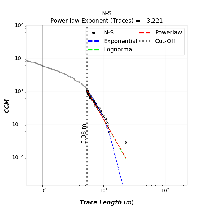
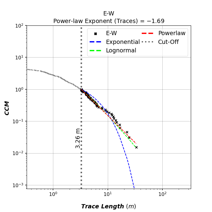
Set-wise length distribution plotting

pprint(KB11_NETWORK.azimuth_set_names)
pprint(KB11_NETWORK.azimuth_set_ranges)

('N-S', 'E-W')
((135, 45), (45, 135))

fits, figs, axes = KB11_NETWORK.plot_trace_azimuth_set_lengths()

• 
•