Though drawing lines on a map might not seem complex, there are still
rules to follow to make the data you produce analyzable without
inconsistencies.
Digitizing lineaments and fractures follows the same process. Usually the
scale of observation and underlying raster data are different but actual
process of digitization is the same. Consequently, any specific
references to “fractures” or “lineaments” are mostly interchangeable,
unless otherwise specified.
The purpose of digitizing is usually creating digital data about
bedrock discontinuities, i.e. fractures and faults. By drawing
along a fracture on a georeferenced picture of an outcrop,
you are documenting the length and orientation of a bedrock feature.
Furthermore, by accurately digitizing relationships between fractures,
you are producing topological information about how fractures
interact and form a network.
Examples and illustrations of fracture digitizing
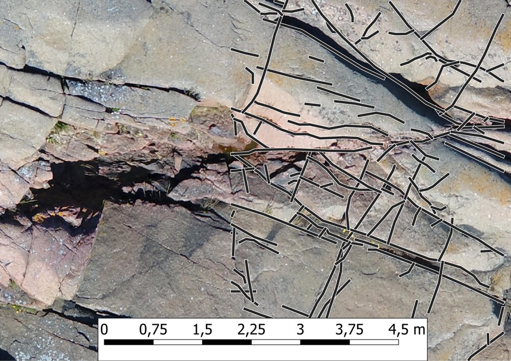
On the left: outcrop photo, on the right: outcrop photo with digitized fractures on top of it
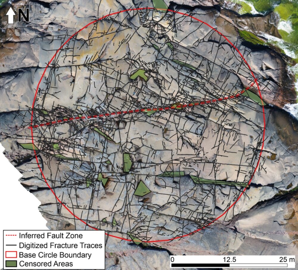
Drone orthomosaic from the northern shores of Åland Islands
with thousands of digitized fractures on top and an inferred
fault zone, i.e. a remotely interpreted potential fault.
1.2. How to digitize fractures and lineaments using QGIS
This guide expects some basic knowledge of geographic information
systems (GIS) and their nomenclature. However, the guide is meant to be
as detailed as necessary for a beginner of QGIS to follow.
This guide has been written for QGIS version 4.0. Some deviation in
terms of different option names and locations is therefore possible
if you are using a different version.
Before opening QGIS, set up an appropriate project directory for
digitization. Create a project directory, with a suitable name, e.g.
brittle_course_fracture_digitization_2026 in a suitable location
under your user directory. E.g. in
C:\Users\<your-username>\projects\ or any other locations you have
used for projects. Set up a suitable directory structure within that
created project directory for
data by creating a data directory with two subdirectories: raster and
vector.
In the following text, I will refer to the project directory with the
name brittle_course_fracture_digitization_2026 and yours may differ.
Tree-view of the project folder:
brittle_course_fracture_digitization_2026
└── data
    ├── raster
    └── vector
Now start up QGIS. Make a new project and save the project file in
brittle_course_fracture_digitization_2026. I would recommend using
the same name for the project file as you have for the project
directory. After saving the project file in the directory, you should
have a new brittle_course_fracture_digitization_2026.qgz file there.
brittle_course_fracture_digitization_2026
├── brittle_course_fracture_digitization_2026.qgz
└── data
    ├── raster
    └── vector
The project coordinate reference system (CRS) should be set to a metric coordinate system
to avoid confusing results from analysis of the finished digitized traces.
If you are in Finland, the recommended CRS is EPSG:3067 (EUREF-FIN / TM35FIN(E,N) - Finland).
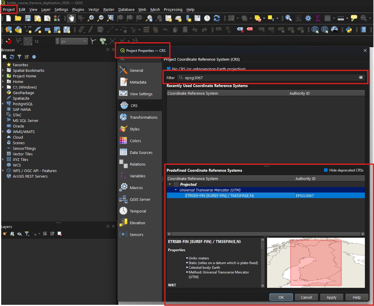
To check and set it, go to Project -> Properties -> CRS. Use
Filter to search for EPSG:3067 and select it. Then click OK
to save the setting.
Screenshot of CRS selection screen
Project coordinate selection window with EPSG:3067 selected.
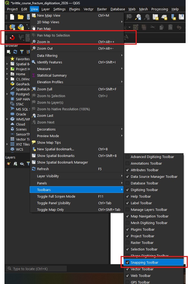
The topological editing tool needs to be added to the toolbar for easy
access. Go to View -> Toolbars and toggle Snappingtoolbar
on.
Screenshot of enabling the QGIS snapping toolbar
Toggle the Snappingtoolbar on, if it is not already. In the
image it is toggled on. It should appear where the upper red
rectangle shows (or within the toolbar somewhere else).
Moving the raster data you are going to use to the data/rasters/
folder of the project directory is recommended as the data will then be
easily accessible in QGIS.
Note
If you use the same raster data in multiple projects, it might be
better to store it in a central location rather than copying it to
each individual project folder, as the raster data itself is never
edited during digitization.
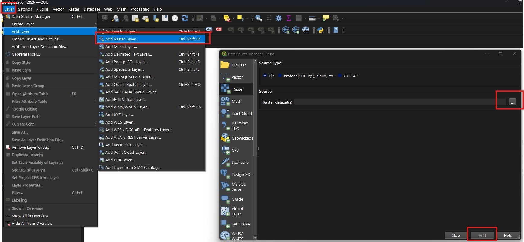
To add raster data into QGIS, go to Layer -> AddLayer ->
AddRasterLayer and select your raster file, which usually has a
.tif or .tiff extension, and click Add to add it to the project.
Adding raster data in QGIS
After choosing the raster file, click Add to add it to the project.
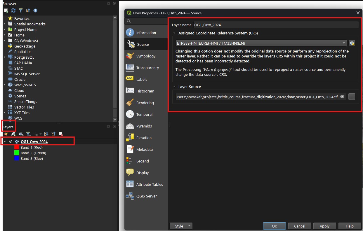
Check that the added raster data uses the same CRS as the project. Right
click on the layer in the Layers tab, click Properties. In the
LayerProperties window, go to Source and check the coordinate
system and change it to the project coordinate system, if necessary.
Screenshot of checking raster layer settings for CRS
Check the CRS in the area indicated by red rectangle.
The rasters can cover large areas and digitizing the whole extent might
not be needed. Consequently, it is a good idea to create a preliminary
target area for digitizing at this point.
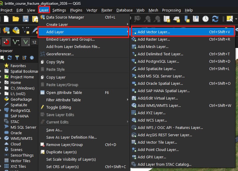
If you have an existing target area layer available, go to
Layer -> AddLayer -> AddVectorLayer. Add the
target area layer similarly to the raster data.
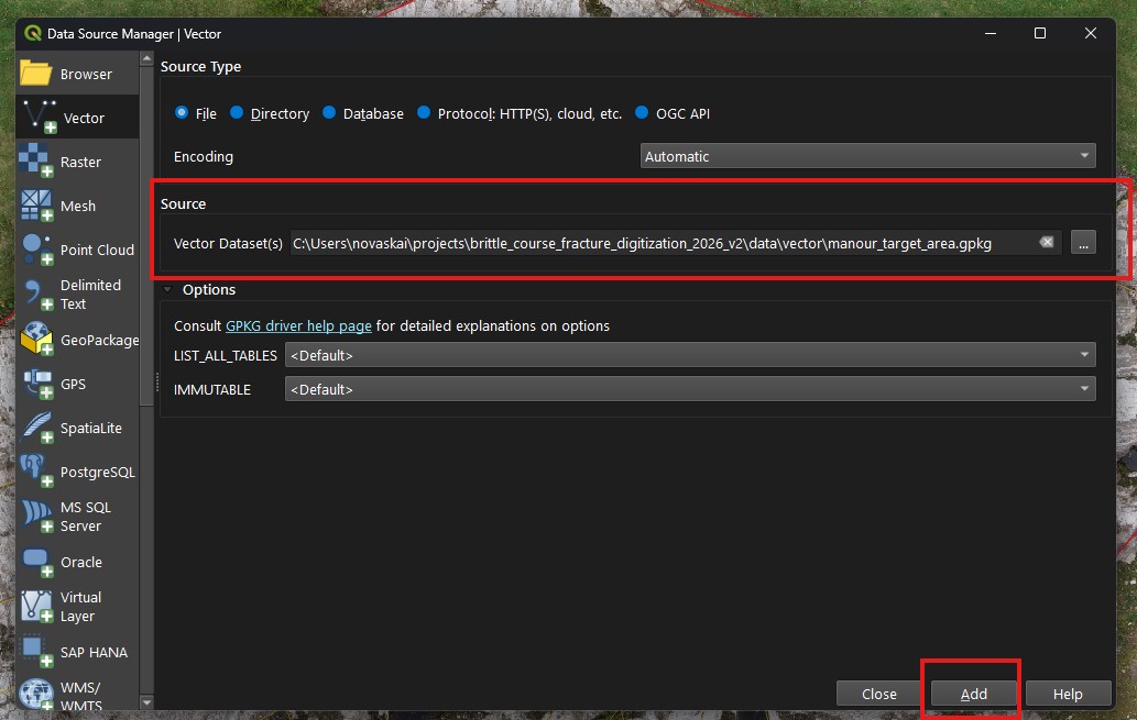
Screenshot of adding existing vector data (such as a target area)
Use AddVectorLayer to add existing, e.g., trace and area
layer data.
Click on the three dots on the right side to select a file.
Default settings are usually okay. After clicking Add,
you might get prompted to choose layer(s) from the vector
database. If there is only one, usually you want to
add it.
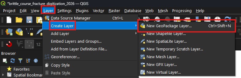
If you do not have an existing target area, create a new polygon vector
layer for the target area by going to Layer -> Createlayer ->
NewGeoPackageLayer.
Screenshot of navigating to NewGeoPackageLayer option
Usage of GeoPackages for storing vector data is recommended due to their
high compatibility and single-file database structure.
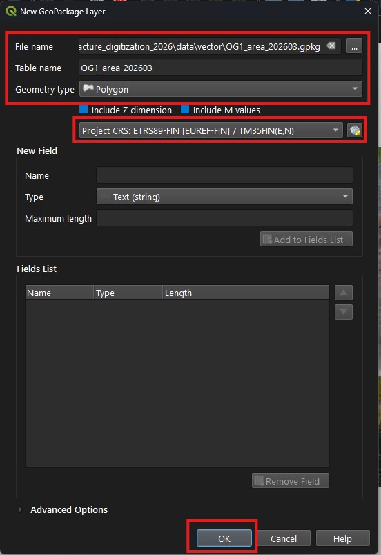
Screenshot of vector layer creation screen with options selected for creating a GeoPackage file for storing target area Polygon data.
Please carefully check 1. that the Tablename is the same as
the filename, without the extension (.gpkg) as seen in
Filename, 2. Geometrytype is Polygon and 3. the CRS
is the same as the project.
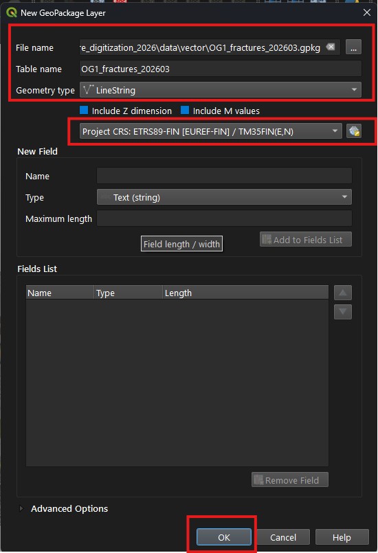
Create a new LineString layer for the traces to be digitized.
At its simplest, the trace layer can only consist of the trace geometries
without any attribute information. When creating your trace layer, select LineString as the geometry type.
Screenshot of vector layer creation screen with options selected for creating a GeoPackage file for storing LineString trace data.
Please carefully check 1. that the Tablename is the same as
the filename, without the extension (.gpkg) as seen in
Filename, 2. Geometrytype is LineString and 3. the CRS
is the same as the project.
Note
Avoid using MultiLineString geometry type. If your lines are
accidentally stored as MultiLineStrings, use QGIS’s “Explode Lines”
tool (Processing Toolbox > Vector geometry > Explode lines) to
convert them to individual LineStrings.
1.2.3. Digitizing fracture and lineament traces in QGIS
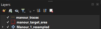
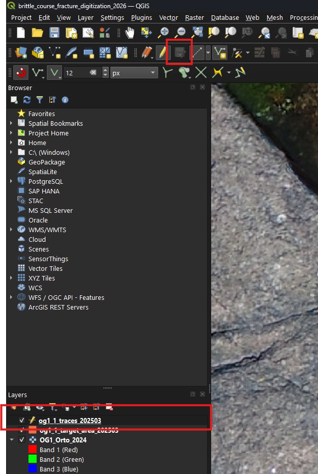
QGIS determines what gets shown on top of what layer in the ordering of
layers in the Layers tab. Make sure the raster layer is at the
bottom, target area layer is on top of it and the layer with the traces
you are digitizing is at the top.
Screenshot of Layers tab with layers organized
Order of target area and traces is not so important.
Orthomosaics, or pictures of outcrops in general, are RGB images
where additional styling is usually not required. However, when
digitizing lineaments using, e.g., digital elevation model (DEM)
data, you might need to configure styling.
The target area is defined by polygon(s). By default, QGIS styles them
with a single color fill, i.e., they mask the layers beneath them.
You can change the styling in the Symbology section, accessed by right
clicking the layer in the Layers tab and selecting Properties.
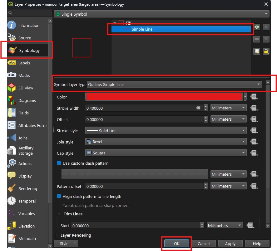
Setting style for target area layer
Click Symbology, then, if SimpleFill (or another fill type)
is being currently used, click it. Then change the
Symbollayertype to Outline:SimpleLine to only show the
boundary of the polygon.
To make digitizing easier, you can try adjusting the trace styles.
Changing the color is particularly helpful for ensuring your work stands
out against the underlying raster layer.
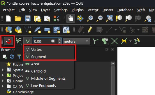
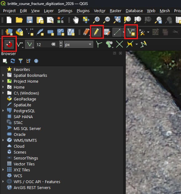
Click the magnet icon in the QGIS toolbar or go to Project > Snapping
Options. Set snapping to “Vertex” and “Segment” for your trace layer,
and choose a small snapping tolerance (e.g., 12 px). Snapping helps
to ensure that traces precisely abut, i.e. endpoint of one trace is
exactly along a segment or on top of a vertex of another trace, to other
traces, which is important for accurate topological network analysis.
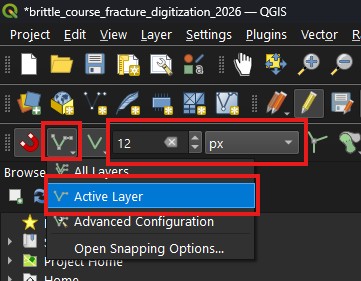
Configuring snapping in the toolbar
Toggle EnableSnapping and set snapping to Vertex and Segment.
1. Configure that new features snap to ActiveLayer so that when
you create new features, they only snap to features in the same
layer. 2. Set SnappingTolerance to 12 px. This determines
how far the cursor will try to snap to old features when creating new
ones.
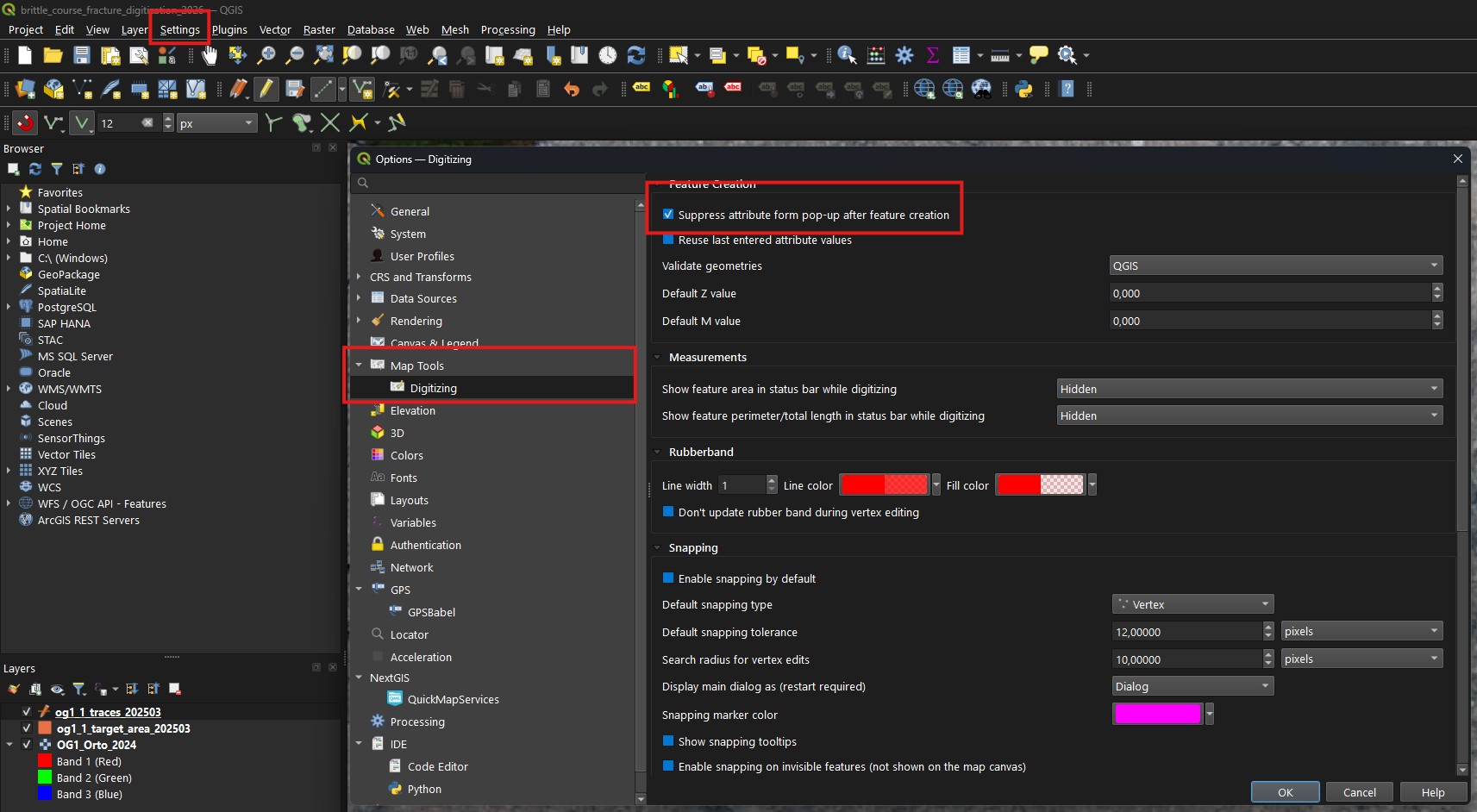
Before starting to digitize traces, you can disable the pop-up that
appears for inputting attribute data after each feature is digitized.
Go to Settings -> Options -> MapTools -> Digitizing.
Check Suppressattributeform... to disable the pop-up.
Suppressing attribute form
Toggle Suppressattributeform... on to disable the pop-up.
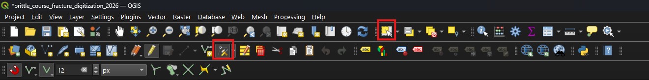
To start digitizing new features, make sure you have selected the trace layer
in the Layers tab. Next, put ToggleEditing toggle on. To create a new
feature, click on AddLineFeature button. Click on the map to create a vertex,
then click again to connect the vertices, and continue digitizing from
one end of the lineament or fracture to the other end. If either end of the fracture
seems to abut another fracture
Digitizing new features
Toggle editing (pen icon) on, then click the create feature button.
Make sure that snapping is turned on (magnet icon).
Remember to save layer changes. You can check if you have unsaved
changes from the Layers tab or from the save button itself.
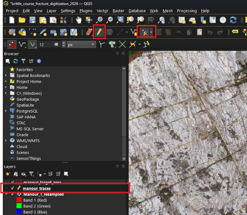
It is often necessary to modify already digitized features due to
reinterpretation and to match them with other digitized fractures. To
start modifying, start editing the layer similarly to when creating new
traces. While editing traces, there are two tools you usually want
to use the most: SelectFeaturesbyAreaorSingleClick and
VertexTool. Use the select tool to select existing traces.
You can then, e.g., delete them. Selecting will also highlight the
vertices of the trace, allowing easier selection with the VertexTool.
Screenshot displaying location of Select... and VertexTool
Usually you want to use select first to highlight vertices and the
trace, then edit it with the vertex tool. Note that the vertex tool
will also allow edits to non-selected traces.
Click on VertexTool to start editing vertices and segments of
traces. Now when moving your cursor above traces, you should see their
vertices highlighted. To modify a single vertex, click on it. You can
then move it and the trace will be modified to fit the new vertex. To
add a new vertex between two existing vertices, click along the trace
somewhere where there is no vertex between the two vertices. To
continue a trace, click on the plus-symbol at either end of the trace to
start appending vertices.
Note
When editing traces, you might accidentally cause another trace to no
longer abut the modified trace. You can avoid this by adding a
vertice along the modified trace at the endpoint of fracture abutting
the modified trace.
Screenshot where layer is in edit mode and vertex tool is highlighted
Toggle editing (pen icon) on, then click the vertex button.
Make sure that snapping is turned on (magnet icon) also when editing.
Note
When editing, sometimes the error or errors can be difficult to spot.
Instead of trying to find the specific error along a trace or in the
intersection of multiple traces, it might be easier to delete the
existing traces that have errors and digitize them again.
1.3. How to digitize fractures and lineaments using ArcGIS Pro
For illustrations of the common digitizing errors, go to the
Validation errors page. Some general tips below.
Avoid unintended intersections
Do not let more than two lines intersect at a single point. If
multiple lines cross at one spot, edit them so only two intersect.
Prevent self-intersections and duplicate lines
Make sure each line does not cross itself.
Avoid drawing duplicate lines directly on top of each other. If
you find duplicates, delete them.
Do not end two traces at the same endpoint (V-node)
You might accidentally create these kind of errors if you do not
make sure that when you continue an existing trace, you actually
extend it rather than creating a new trace from the endpoint of
the existing trace (See
Modifying existing traces)
Trace length and target area
If you have created a target area to control where you are going
to digitize, make sure you do not stop your traces at the
boundary. Rather, continue them outside the boundary as far as
they can be interpreted to continue. Otherwise trace lengths might
be improperly samples. Furthermore, the target area you currently
have might be extended in the future.
1.5. How to collect metadata for digitized fractures
If you want to validate your data using fractopo, you can do so
using the command-line interface (See fractopo), using Python
code in a script or a notebook (See
Notebook - Fractopo – KB11 Trace Data Validation) or using the validation web interface if you have it available (See Validation).