Usage Guide
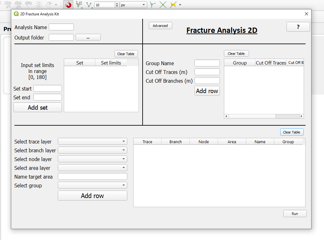
The whole functionality of the tool is accessible through a single GUI window within QGIS. In this window the data to analyze must be inputted along with the output folder, names, etc.

The GUI window of Fracture Analysis Kit 2D. Hover over elements in QGIS such as buttons and prompts for short help texts and example inputs.
Outputs
- Analysis Name
Name the current analysis. This will be used in the folder structure where plots are saved.
- Output folder
Folder where analysis results are saved to.
Set limits
This table is used to input set ranges/limits for the analysis. This can be left blank in which case default sets are used.
E.g. Set start = 10 -> Set end = 30 -> Press **Add set** -> New set with the label **1** will be made.
Repeat for more sets with incremental numbering (1, 2, 3, etc.)
Grouping data and cut-offs for length distribution modelling
If you have fracture data from multiple scales of observation, each scale can be grouped here and the scale-compassing datasets can be compared with each other e.g. in powerlaw length distribution modelling.
Each group also shares a cut-off value (used in powerlaw modelling) for trace and branch data. Currently the powerlaw modelling done by the powerlaw Python package does two analyses:
powerlaw analysis with user inputted values (given here)
powerlaw analysis with automatically derived cut-offs
E.g. Group Name = KB -> Cut Off Traces (m) = 1.8 -> Cut Off Branches (m) = 1.6 -> Press **Add row**
Input data table
The input data table consists of rows each of which contain a trace, branch, node and area dataset along with a name (e.g. KB11) and a group. All must be given for each row to perform the analysis.
Branch and node data can be acquired with NetworkGT using the trace and target area data.
Miscellanous
- Advanced
The plugin comes with a config.py Python file wherein some manual setup is possible. Most importantly the analyses which to perform can be chosen. On default all analyses are done which can be computationally intensive.
- ?
Opens this help documentation locally.